How to Install Django 1.10 on Ubuntu 16.04

In this tutorial, we will install Django 1.10 on a Ubuntu 16.04 server. Django can be installed on a server in many ways, in this tutorial, I will show you 3 different ways to install Django:

1. Django installation with pip.
2. Install Django with virtualenv.
3. Install Django fron it's github repository.

When the Django installation is done, I will show you the first steps to start a new project with the Django web framework.
Django is a web application framework written in python that follows the MVC (Model-View-Controller) architecture, it is available for free and released under an open source license. It is fast and designed to help developers get their application online as quickly as possible. Django helps developers to avoid many common security mistakes like SQL Injection, XSS, CSRF and clickjacking. Django is maintained by the Django Software Foundation and used by many big technology companies, government, and other organizations. Some large websites like Pinterest, Mozilla, Instagram, Discuss, The Washington Post etc. are developed with Django.

Prerequisites

• Ubuntu 16.04 - 64bit.
• Root privileges.

Step 1 - Setup python 3 as Default Python version

We will configure python 3 before we start with the Django installation.
On my Ubuntu machine, there are two versions of python available, python2.7 as default python version and python3. In this step, we will change the default python version to python 3.
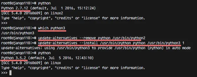
Check the python version:

python

Result:

python

Python 2.7.12 (default, Jul  1 2016, 15:12:24)
[GCC 5.4.0 20160609] on linux2
Type "help", "copyright", "credits" or "license" for more information.
>>>

So the default python is 2.7 at the moment.
Next, remove default python 2 and change the default to python 3 with the 'update-alternatives' command:

update-alternatives --remove python /usr/bin/python2
update-alternatives --install /usr/bin/python python /usr/bin/python3

Now check again the python version:

python

Result:

python

Python 3.5.2 (default, Jul  5 2016, 12:43:10)
[GCC 5.4.0 20160609] on linux
Type "help", "copyright", "credits" or "license" for more information.
>>>

Step 2 - Install Django

In this step, I will show you 3 ways to install Django. Please follow either chpater 2.1, 2.2 or 2.3 to install Django but not all 3 options at the same time :)

2.1. Install Django with Pip

Pip is a package management system for python. Python has a central package repository from which we can download the python package. It's called Python Package Index (PyPI).
In this tutorial, we will use python 3 for django as recommended by the django website. Next, we will install pip for python 3 from the ubuntu repository with this apt command:

apt-get install python3-pip

The installation will add a new binary file called 'pip3'. To make it easier to use pip, I will create a symlink for pip3 to pip:

which pip3
ln -s /usr/bin/pip3 /usr/bin/pip

Now check the version :

pip -V

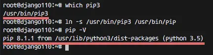
The pip installation is done. Now we can use the pip command to install python packages. Let's install django on our server with pip command below:

pip install django==1.10

Note:
We set django==1.10 to get a specific version. If you want a different version, just change the number e.g. to django==1.9 etc.
If you have an error about the locale settings, run the command below to reconfigure the locale settings:

export LANGUAGE=en_US.UTF-8
export LANG=en_US.UTF-8
export LC_ALL=en_US.UTF-8
locale-gen en_US.UTF-8
dpkg-reconfigure locales

When the installation is done, check the django version with the command below:

django-admin --version

Alternatively, we can use command below:

python
import django
print(django.get_version())

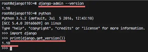
Django 1.10 has been installed on the system with pip. Proceed with chapter 3.

2.2. Install Django with Virtualenv

Virtualenv is a python environment builder, it is used to create isolated python environments. We can choose the version of python that will be install in the virtualenv environment. This is very useful for developers, they can run and develop an application with different python versions and different environments on one OS.
Virtualenv is available on PyPI, we can install it with the pip command:

pip install virtualenv

Now we can use the virtualenv command to create a new environment with python3 as default python version. So let's create a new environment "mynewenv" with python3 as the python version and pip3 for the django installation.

virtualenv --python=python3 mynewenv

Note :
--python=python3 is a binary file for python 3.
mynewenv is the name of the environment.
The command will create a new directory called 'mynewenv' which contains the directories bin, include and lib.
The virtualenv has been created, now let's log into the new environment with the command below:

source mynewenv/bin/activate

If you do not have the source command, you can run this command instead:

. mynewenv/bin/activate

Note: If you want to get out from the virtual environment, use the command 'deactivate'.
Now check the pip version:

pip -V

Pip will be automatically installed inside the virtual environment.
Next, install django in thevirtual environment that we've created:

pip install django==1.10

When the installation finished, check the Django installation:

django-admin --version

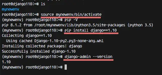
Django 1.10 has been successfully installed inside our virtual environment. Proceed with chapter 3.

2.3. Install Django from Git Repository

In this chapter, we will install the Django web frame work inside the system, not in a virtual environment. I will show you how to install it manually from the Django Git repository. Make sure you have git installed on your server. If you don't have git, install it with the command below:

apt-get install git -y

Next, create a new python virtual environment and activate it:

virtualenv --python=python3 django-git
source django-git/bin/activate

Then clone the django git repository with the command below:

cd django-git
git clone git://github.com/django/django django-dev

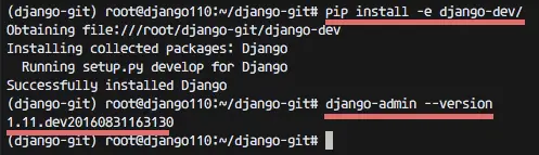
Install django with this pip command:

pip install -e django-dev/

-e =  Install a package in editable mode or a local package. In this chapter, we install Django from the local code that we've cloned.


When the installation process is done, let's check the Django version on the server:

django-admin --version
1.11.dev20160831163130

We see the django 1.11 dev version.
The manual Django installation is finished.

Step 3 - Create you First Project with Django

In this step, we will install django inside a virtual environment and then start our first project with django.
Install virtualenv on the server and create a new environment named 'firstdjango' :

pip install virtualenv
virtualenv --python=python3 firstdjango

Now go to the firstdjango directory and activate the virtual envonment, then install django with the pip command:

cd firstdjango/
source bin/activate
pip install django==1.10

Next, create a new project called 'myblog' with the django-admin command:

django-admin startproject myblog

It will create a new directory myblog that contains the django files:

ll myblog

-rwxr-xr-x 1 root root  249 Sep 06 09:01 manage.py*
drwxr-xr-x 2 root root 4096 Sep 06 09:01 myblog/

Go to the myblog directory and run the 'manage.py' file :

cd myblog/
python manage.py runserver

The runserver option will create a HTTP connection with python on localhost IP and port 8000. If your development environment is on a separate server, as in my example here I'm using an Ubuntu server with I : 192.168.1.9, you can use the server IP so you can access Django from outside of the server.

python manage.py runserver 192.168.1.9:8000

Now check from your browser: 192.168.1.9:8000

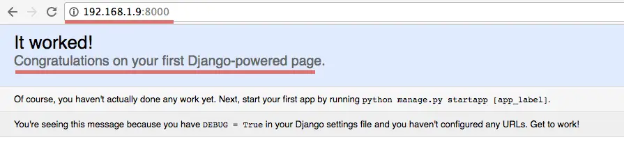
The Django default page is working and inside the server, you can look at the access log:

[31/Aug/2016 17:04:40] "GET / HTTP/1.1" 200 1767

Next, we will configure the Django admin. Django will automatically generate the database for a superuser. Before we create the superuser, run the command below:

python manage.py migrate

migrate: make adds the models (adding fields, deleting etc.) into the database scheme, the default database is sqlite3.
Now create the admin/superuser:

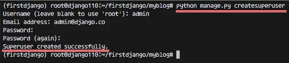
python manage.py createsuperuser

Username (leave blank to use 'root'): admin
Email address: admin@mydjango.co
Password:
Password (again):
Superuser created successfully.

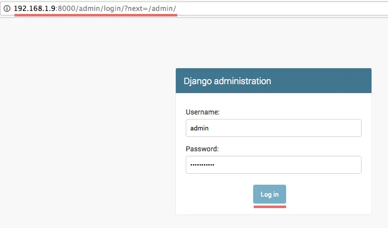
The Django super user has been added, now you can execute the runserver command, then go to the browser and visit the django admin page:

python manage.py runserver 192.168.1.9:8000

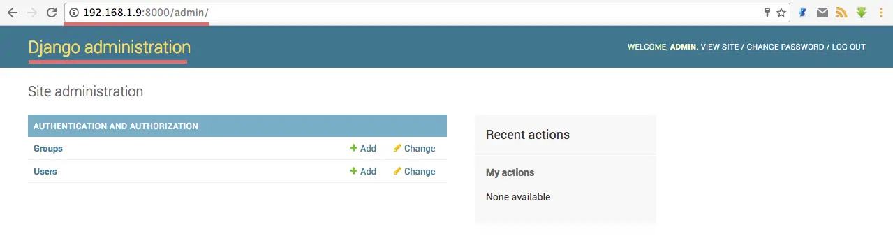
Visit Django admin page: 192.168.1.9:8000/admin/. Login with username admin and your password, you will see the admin page:
Django admin login page.

The Django admin dashboard.

Django has been successfully installed inside a virtual environment and we've created a sample Django project named 'firstdjango'.

Conclusion

Django is a web framework based on the Python programming language, it is released as free software under an open source license and maintained by the Django Software Foundation. Django is very fast and allows it to build web applications rapidly. Django is a web framework that uses the MVC (Model-View-Controller) paradigm. We can install Django on a server with the pip command, in a virtual environment with virtualenv and directly from the Django git repository.

What is iBeacon? A Guide to Beacons

What is iBeacon? What are iBeacons? 

The term iBeacon and Beacon are often used interchangeably. iBeacon is the name for Apple’s technology standard, which allows Mobile Apps (running on both iOS and Android devices) to listen for signals from beacons in the physical world and react accordingly. In essence, iBeacon technology allows Mobile Apps to understand their position on a micro-local scale, and deliver hyper-contextual content to users based on location. The underlying communication technology is Bluetooth Low Energy.

iBeacon Contextual, Hyperlocal Content

What is Bluetooth Low Energy (BLE)?

Bluetooth Low Energy is a wireless personal area network technology used for transmitting data over short distances. As the name implies, it’s designed for low energy consumption and cost, while maintaining a communication range similar to that of its predecessor, Classic Bluetooth.

How is BLE different from Regular Bluetooth?

• Power Consumption: Bluetooth LE, as the name hints, has low energy requirements. It can last up to 3 years on a single coin cell battery.
• Lower Cost: BLE is 60-80% cheaper than traditional Bluetooth.
• Application: BLE is ideal for simple applications requiring small periodic transfers of data. Classic Bluetooth is preferred for more complex applications requiring consistent communication and more data throughput.

How does BLE communication work?

BLE communication consists primarily of “Advertisements”, or small packets of data, broadcast at a regular interval by Beacons or other BLE enabled devices via radio waves.

BLE Advertising is a one-way communication method. Beacons that want to be “discovered” can broadcast, or “Advertise” self-contained packets of data in set intervals. These packets are meant to be collected by devices like smartphones, where they can be used for a variety of smartphone applications to trigger things like push messages, app actions, and prompts.

Apple’s iBeacon standard calls for an optimal broadcast interval of 100 ms.  Broadcasting more frequently uses more battery life but allows for quicker discovery by smartphones and other listening devices.

Standard BLE has a broadcast range of up to 100 meters, which make Beacons ideal for indoor location tracking and awareness.

Source: Nerdery

How does iBeacon use BLE communication?

With iBeacon, Apple has standardized the format for BLE Advertising. Under this format, an advertising packet consists of four main pieces of information.

UUID: This is a 16 byte string used to differentiate a large group of related beacons. For example, if Coca-Cola maintained a network of beacons in a chain of grocery stores, all Coca-Cola beacons would share the same UUID. This allows Coca-Cola’s dedicated smartphone app to know which beacon advertisements come from Coca-Cola-owned beacons.

Major: This is a 2 byte string used to distinguish a smaller subset of beacons within the larger group. For example, if Coca-Cola had four beacons in a particular grocery store, all four would have the same Major. This allows Coca-Cola to know exactly which store its customer is in.

Minor: This is a 2 byte string meant to identify individual beacons. Keeping with the Coca-Cola example, a beacon at the front of the store would have its own unique Minor. This allows Coca-Cola’s dedicated app to know exactly where the customer is in the store.

Tx Power: This is used to determine proximity (distance) from the beacon. How does this work? TX power is defined as the strength of the signal exactly 1 meter from the device. This has to be calibrated and hardcoded in advance. Devices can then use this as a baseline to give a rough distance estimate. 

Example:

A beacon broadcasts the following packet

UUID: 12345678910245

Major: 22

Minor: 2

A device receiving this packet would understand it’s from the Coca-Cola Beacon (UUID) in the Target on 1^st Street (Major) at the front of the store (Minor). 

How iBeacons Work (Source: estimote.com)

Why is iBeacon a Big Deal? 

With an iBeacon network, any brand, retailer, app, or platform will be able to understand exactly where a customer is in the brick and mortar environment. This provides an opportunity to send customers highly contextual, hyper-local, meaningful messages and advertisements on their smartphones.

The typical scenario looks like this. A consumer carrying a smartphone walks into a store. Apps installed on a consumer’s smartphone listen for iBeacons. When an app hears an iBeacon, it communicates the relevant data (UUID, Major, Minor, Tx) to its server, which then triggers an action. This could be something as simple as a push message [“Welcome to Target! Check out Doritos on Aisle 3!”], and could include other things like targeted advertisements, special offers, and helpful reminders [“You’re out of Milk!”]. Other potential applications include mobile payments and shopper analytics and implementation outside of retail, at airports, concert venues, theme parks, and more. The potential is limitless.

This technology should bring about a paradigm shift in the way brands communicate with consumers. iBeacon provides a digital extension into the physical world. We’re excited to see where iBeacon technology goes in the next few years.

Implement Simple Linear Regression With Python

Linear regression is a prediction method that is more than 200 years old.
Simple linear regression is a great first machine learning algorithm to implement as it requires you to estimate properties from your training dataset, but is simple enough for beginners to understand.
In this tutorial, you will discover how to implement the simple linear regression algorithm from scratch in Python.
After completing this tutorial you will know:

• How to estimate statistical quantities from training data.
• How to estimate linear regression coefficients from data.
• How to make predictions using linear regression for new data.

Let’s get started.

How To Implement Simple Linear Regression From Scratch With Python

Photo by Kamyar Adl, some rights reserved.

Description

This section is divided into two parts, a description of the simple linear regression technique and a description of the dataset to which we will later apply it.

Simple Linear Regression

Linear regression assumes a linear or straight line relationship between the input variables (X) and the single output variable (y).
More specifically, that output (y) can be calculated from a linear combination of the input variables (X). When there is a single input variable, the method is referred to as a simple linear regression.
In simple linear regression we can use statistics on the training data to estimate the coefficients required by the model to make predictions on new data.
The line for a simple linear regression model can be written as:

y = b0 + b1 * x

1	y = b0 + b1 * x

where b0 and b1 are the coefficients we must estimate from the training data.
Once the coefficients are known, we can use this equation to estimate output values for y given new input examples of x.
It requires that you calculate statistical properties from the data such as mean, variance and covariance.
All the algebra has been taken care of and we are left with some arithmetic to implement to estimate the simple linear regression coefficients.
Briefly, we can estimate the coefficients as follows:

B1 = sum((x(i) - mean(x)) * (y(i) - mean(y))) / sum( (x(i) - mean(x))^2 ) B0 = mean(y) - B1 * mean(x)

1 2	B1 = sum((x(i) - mean(x)) * (y(i) - mean(y))) / sum( (x(i) - mean(x))^2 ) B0 = mean(y) - B1 * mean(x)

where the i refers to the value of the ith value of the input x or output y.
Don’t worry if this is not clear right now, these are the functions will implement in the tutorial.

Swedish Insurance Dataset

We will use a real dataset to demonstrate simple linear regression.
The dataset is called the “Auto Insurance in Sweden” dataset and involves predicting the total payment for all the claims in thousands of Swedish Kronor (y) given the total number of claims (x).
This means that for a new number of claims (x) we will be able to predict the total payment of claims (y).
Here is a small sample of the first 5 records of the dataset.

108,392.5 19,46.2 13,15.7 124,422.2 40,119.4

1 2 3 4 5

108,392.5 19,46.2 13,15.7 124,422.2 40,119.4

Using the Zero Rule algorithm (that predicts the mean value) a Root Mean Squared Error or RMSE of about 72.251 (thousands of Kronor) is expected.
Below is a scatter plot of the entire dataset.

Swedish Insurance Dataset

You can download the raw dataset from here or here.
Save it to a CSV file in your local working directory with the name “insurance.csv“.
Note, you may need to convert the European “,” to the decimal “.”. You will also need change the file from white-space-separated variables to CSV format.

Tutorial

This tutorial is broken down into five parts:

1. Calculate Mean and Variance.
2. Calculate Covariance.
3. Estimate Coefficients.
4. Make Predictions.
5. Predict Insurance.

These steps will give you the foundation you need to implement and train simple linear regression models for your own prediction problems.

1. Calculate Mean and Variance

The first step is to estimate the mean and the variance of both the input and output variables from the training data.
The mean of a list of numbers can be calculated as:

mean(x) = sum(x) / count(x)

1	mean(x) = sum(x) / count(x)

Below is a function named mean() that implements this behavior for a list of numbers.

# Calculate the mean value of a list of numbers def mean(values): return sum(values) / float(len(values))

1 2 3

# Calculate the mean value of a list of numbers def mean(values): return sum(values) / float(len(values))

The variance is the sum squared difference for each value from the mean value.
Variance for a list of numbers can be calculated as:

variance = sum( (x - mean(x))^2 )

1	variance = sum( (x - mean(x))^2 )

Below is a function named variance() that calculates the variance of a list of numbers. It requires the mean of the list to be provided as an argument, just so we don’t have to calculate it more than once.

# Calculate the variance of a list of numbers def variance(values, mean): return sum([(x-mean)**2 for x in values])

1 2 3

# Calculate the variance of a list of numbers def variance(values, mean): return sum([(x-mean)**2 for x in values])

We can put these two functions together and test them on a small contrived dataset.
Below is a small dataset of x and y values.
NOTE: delete the column headers from this data if you save it to a .CSV file for use with the final code example.

x, y 1, 1 2, 3 4, 3 3, 2 5, 5

1 2 3 4 5 6

x, y 1, 1 2, 3 4, 3 3, 2 5, 5

We can plot this dataset on a scatter plot graph as follows:

Small Contrived Dataset For Simple Linear Regression

We can calculate the mean and variance for both the x and y values in the example below.

# Estimate Mean and Variance # Calculate the mean value of a list of numbers def mean(values): return sum(values) / float(len(values)) # Calculate the variance of a list of numbers def variance(values, mean): return sum([(x-mean)**2 for x in values]) # calculate mean and variance dataset = [[1, 1], [2, 3], [4, 3], [3, 2], [5, 5]] x = [row[0] for row in dataset] y = [row[1] for row in dataset] mean_x, mean_y = mean(x), mean(y) var_x, var_y = variance(x, mean_x), variance(y, mean_y) print('x stats: mean=%.3f variance=%.3f' % (mean_x, var_x)) print('y stats: mean=%.3f variance=%.3f' % (mean_y, var_y))

1 2 3 4 5 6 7 8 9 10 11 12 13 14 15 16 17 18

# Estimate Mean and Variance # Calculate the mean value of a list of numbers def mean(values): return sum(values) / float(len(values)) # Calculate the variance of a list of numbers def variance(values, mean): return sum([(x-mean)**2 for x in values]) # calculate mean and variance dataset = [[1, 1], [2, 3], [4, 3], [3, 2], [5, 5]] x = [row[0] for row in dataset] y = [row[1] for row in dataset] mean_x, mean_y = mean(x), mean(y) var_x, var_y = variance(x, mean_x), variance(y, mean_y) print('x stats: mean=%.3f variance=%.3f' % (mean_x, var_x)) print('y stats: mean=%.3f variance=%.3f' % (mean_y, var_y))

Running this example prints out the mean and variance for both columns.

x stats: mean=3.000 variance=10.000 y stats: mean=2.800 variance=8.800

1 2	x stats: mean=3.000 variance=10.000 y stats: mean=2.800 variance=8.800

This is our first step, next we need to put these values to use in calculating the covariance.

2. Calculate Covariance

The covariance of two groups of numbers describes how those numbers change together.
Covariance is a generalization of correlation. Correlation describes the relationship between two groups of numbers, whereas covariance can describe the relationship between two or more groups of numbers.
Additionally, covariance can be normalized to produce a correlation value.
Nevertheless, we can calculate the covariance between two variables as follows:

covariance = sum((x(i) - mean(x)) * (y(i) - mean(y)))

1	covariance = sum((x(i) - mean(x)) * (y(i) - mean(y)))

Below is a function named covariance() that implements this statistic. It builds upon the previous step and takes the lists of x and y values as well as the mean of these values as arguments.

# Calculate covariance between x and y def covariance(x, mean_x, y, mean_y): covar = 0.0 for i in range(len(x)): covar += (x[i] - mean_x) * (y[i] - mean_y) return covar

1 2 3 4 5 6

# Calculate covariance between x and y def covariance(x, mean_x, y, mean_y): covar = 0.0 for i in range(len(x)): covar += (x[i] - mean_x) * (y[i] - mean_y) return covar

We can test the calculation of the covariance on the same small contrived dataset as in the previous section.
Putting it all together we get the example below.

# Calculate Covariance # Calculate the mean value of a list of numbers def mean(values): return sum(values) / float(len(values)) # Calculate covariance between x and y def covariance(x, mean_x, y, mean_y): covar = 0.0 for i in range(len(x)): covar += (x[i] - mean_x) * (y[i] - mean_y) return covar # calculate covariance dataset = [[1, 1], [2, 3], [4, 3], [3, 2], [5, 5]] x = [row[0] for row in dataset] y = [row[1] for row in dataset] mean_x, mean_y = mean(x), mean(y) covar = covariance(x, mean_x, y, mean_y) print('Covariance: %.3f' % (covar))

1 2 3 4 5 6 7 8 9 10 11 12 13 14 15 16 17 18 19 20

# Calculate Covariance # Calculate the mean value of a list of numbers def mean(values): return sum(values) / float(len(values)) # Calculate covariance between x and y def covariance(x, mean_x, y, mean_y): covar = 0.0 for i in range(len(x)): covar += (x[i] - mean_x) * (y[i] - mean_y) return covar # calculate covariance dataset = [[1, 1], [2, 3], [4, 3], [3, 2], [5, 5]] x = [row[0] for row in dataset] y = [row[1] for row in dataset] mean_x, mean_y = mean(x), mean(y) covar = covariance(x, mean_x, y, mean_y) print('Covariance: %.3f' % (covar))

Running this example prints the covariance for the x and y variables.

Covariance: 8.000

1	Covariance: 8.000

We now have all the pieces in place to calculate the coefficients for our model.

3. Estimate Coefficients

We must estimate the values for two coefficients in simple linear regression.
The first is B1 which can be estimated as:

B1 = sum((x(i) - mean(x)) * (y(i) - mean(y))) / sum( (x(i) - mean(x))^2 )

1	B1 = sum((x(i) - mean(x)) * (y(i) - mean(y))) / sum( (x(i) - mean(x))^2 )

We have learned some things above and can simplify this arithmetic to:

B1 = covariance(x, y) / variance(x)

1	B1 = covariance(x, y) / variance(x)

We already have functions to calculate covariance() and variance().
Next, we need to estimate a value for B0, also called the intercept as it controls the starting point of the line where it intersects the y-axis.

B0 = mean(y) - B1 * mean(x)

1	B0 = mean(y) - B1 * mean(x)

Again, we know how to estimate B1 and we have a function to estimate mean().
We can put all of this together into a function named coefficients() that takes the dataset as an argument and returns the coefficients.

# Calculate coefficients def coefficients(dataset): x = [row[0] for row in dataset] y = [row[1] for row in dataset] x_mean, y_mean = mean(x), mean(y) b1 = covariance(x, x_mean, y, y_mean) / variance(x, x_mean) b0 = y_mean - b1 * x_mean return [b0, b1]

1 2 3 4 5 6 7 8

# Calculate coefficients def coefficients(dataset): x = [row[0] for row in dataset] y = [row[1] for row in dataset] x_mean, y_mean = mean(x), mean(y) b1 = covariance(x, x_mean, y, y_mean) / variance(x, x_mean) b0 = y_mean - b1 * x_mean return [b0, b1]

We can put this together with all of the functions from the previous two steps and test out the calculation of coefficients.

# Calculate Coefficients # Calculate the mean value of a list of numbers def mean(values): return sum(values) / float(len(values)) # Calculate covariance between x and y def covariance(x, mean_x, y, mean_y): covar = 0.0 for i in range(len(x)): covar += (x[i] - mean_x) * (y[i] - mean_y) return covar # Calculate the variance of a list of numbers def variance(values, mean): return sum([(x-mean)**2 for x in values]) # Calculate coefficients def coefficients(dataset): x = [row[0] for row in dataset] y = [row[1] for row in dataset] x_mean, y_mean = mean(x), mean(y) b1 = covariance(x, x_mean, y, y_mean) / variance(x, x_mean) b0 = y_mean - b1 * x_mean return [b0, b1] # calculate coefficients dataset = [[1, 1], [2, 3], [4, 3], [3, 2], [5, 5]] b0, b1 = coefficients(dataset) print('Coefficients: B0=%.3f, B1=%.3f' % (b0, b1))

1 2 3 4 5 6 7 8 9 10 11 12 13 14 15 16 17 18 19 20 21 22 23 24 25 26 27 28 29 30

# Calculate Coefficients # Calculate the mean value of a list of numbers def mean(values): return sum(values) / float(len(values)) # Calculate covariance between x and y def covariance(x, mean_x, y, mean_y): covar = 0.0 for i in range(len(x)): covar += (x[i] - mean_x) * (y[i] - mean_y) return covar # Calculate the variance of a list of numbers def variance(values, mean): return sum([(x-mean)**2 for x in values]) # Calculate coefficients def coefficients(dataset): x = [row[0] for row in dataset] y = [row[1] for row in dataset] x_mean, y_mean = mean(x), mean(y) b1 = covariance(x, x_mean, y, y_mean) / variance(x, x_mean) b0 = y_mean - b1 * x_mean return [b0, b1] # calculate coefficients dataset = [[1, 1], [2, 3], [4, 3], [3, 2], [5, 5]] b0, b1 = coefficients(dataset) print('Coefficients: B0=%.3f, B1=%.3f' % (b0, b1))

Running this example calculates and prints the coefficients.

Coefficients: B0=0.400, B1=0.800

1	Coefficients: B0=0.400, B1=0.800

Now that we know how to estimate the coefficients, the next step is to use them.

4. Make Predictions

The simple linear regression model is a line defined by coefficients estimated from training data.
Once the coefficients are estimated, we can use them to make predictions.
The equation to make predictions with a simple linear regression model is as follows:

y = b0 + b1 * x

1	y = b0 + b1 * x

Below is a function named simple_linear_regression() that implements the prediction equation to make predictions on a test dataset. It also ties together the estimation of the coefficients on training data from the steps above.
The coefficients prepared from the training data are used to make predictions on the test data, which are then returned.

def simple_linear_regression(train, test): predictions = list() b0, b1 = coefficients(train) for row in test: yhat = b0 + b1 * row[0] predictions.append(yhat) return predictions

1 2 3 4 5 6 7

def simple_linear_regression(train, test): predictions = list() b0, b1 = coefficients(train) for row in test: yhat = b0 + b1 * row[0] predictions.append(yhat) return predictions

Let’s pull together everything we have learned and make predictions for our simple contrived dataset.
As part of this example, we will also add in a function to manage the evaluation of the predictions called evaluate_algorithm() and another function to estimate the Root Mean Squared Error of the predictions called rmse_metric().
The full example is listed below.

# Standalone simple linear regression example from math import sqrt # Calculate root mean squared error def rmse_metric(actual, predicted): sum_error = 0.0 for i in range(len(actual)): prediction_error = predicted[i] - actual[i] sum_error += (prediction_error ** 2) mean_error = sum_error / float(len(actual)) return sqrt(mean_error) # Evaluate regression algorithm on training dataset def evaluate_algorithm(dataset, algorithm): test_set = list() for row in dataset: row_copy = list(row) row_copy[-1] = None test_set.append(row_copy) predicted = algorithm(dataset, test_set) print(predicted) actual = [row[-1] for row in dataset] rmse = rmse_metric(actual, predicted) return rmse # Calculate the mean value of a list of numbers def mean(values): return sum(values) / float(len(values)) # Calculate covariance between x and y def covariance(x, mean_x, y, mean_y): covar = 0.0 for i in range(len(x)): covar += (x[i] - mean_x) * (y[i] - mean_y) return covar # Calculate the variance of a list of numbers def variance(values, mean): return sum([(x-mean)**2 for x in values]) # Calculate coefficients def coefficients(dataset): x = [row[0] for row in dataset] y = [row[1] for row in dataset] x_mean, y_mean = mean(x), mean(y) b1 = covariance(x, x_mean, y, y_mean) / variance(x, x_mean) b0 = y_mean - b1 * x_mean return [b0, b1] # Simple linear regression algorithm def simple_linear_regression(train, test): predictions = list() b0, b1 = coefficients(train) for row in test: yhat = b0 + b1 * row[0] predictions.append(yhat) return predictions # Test simple linear regression dataset = [[1, 1], [2, 3], [4, 3], [3, 2], [5, 5]] rmse = evaluate_algorithm(dataset, simple_linear_regression) print('RMSE: %.3f' % (rmse))

1 2 3 4 5 6 7 8 9 10 11 12 13 14 15 16 17 18 19 20 21 22 23 24 25 26 27 28 29 30 31 32 33 34 35 36 37 38 39 40 41 42 43 44 45 46 47 48 49 50 51 52 53 54 55 56 57 58 59 60 61 62

# Standalone simple linear regression example from math import sqrt # Calculate root mean squared error def rmse_metric(actual, predicted): sum_error = 0.0 for i in range(len(actual)): prediction_error = predicted[i] - actual[i] sum_error += (prediction_error ** 2) mean_error = sum_error / float(len(actual)) return sqrt(mean_error) # Evaluate regression algorithm on training dataset def evaluate_algorithm(dataset, algorithm): test_set = list() for row in dataset: row_copy = list(row) row_copy[-1] = None test_set.append(row_copy) predicted = algorithm(dataset, test_set) print(predicted) actual = [row[-1] for row in dataset] rmse = rmse_metric(actual, predicted) return rmse # Calculate the mean value of a list of numbers def mean(values): return sum(values) / float(len(values)) # Calculate covariance between x and y def covariance(x, mean_x, y, mean_y): covar = 0.0 for i in range(len(x)): covar += (x[i] - mean_x) * (y[i] - mean_y) return covar # Calculate the variance of a list of numbers def variance(values, mean): return sum([(x-mean)**2 for x in values]) # Calculate coefficients def coefficients(dataset): x = [row[0] for row in dataset] y = [row[1] for row in dataset] x_mean, y_mean = mean(x), mean(y) b1 = covariance(x, x_mean, y, y_mean) / variance(x, x_mean) b0 = y_mean - b1 * x_mean return [b0, b1] # Simple linear regression algorithm def simple_linear_regression(train, test): predictions = list() b0, b1 = coefficients(train) for row in test: yhat = b0 + b1 * row[0] predictions.append(yhat) return predictions # Test simple linear regression dataset = [[1, 1], [2, 3], [4, 3], [3, 2], [5, 5]] rmse = evaluate_algorithm(dataset, simple_linear_regression) print('RMSE: %.3f' % (rmse))

Running this example displays the following output that first lists the predictions and the RMSE of these predictions.

[1.1999999999999995, 1.9999999999999996, 3.5999999999999996, 2.8, 4.3999999999999995] RMSE: 0.693

1 2	[1.1999999999999995, 1.9999999999999996, 3.5999999999999996, 2.8, 4.3999999999999995] RMSE: 0.693

Finally, we can plot the predictions as a line and compare it to the original dataset.

Predictions For Small Contrived Dataset For Simple Linear Regression

5. Predict Insurance

We now know how to implement a simple linear regression model.
Let’s apply it to the Swedish insurance dataset.
This section assumes that you have downloaded the dataset to the file insurance.csv and it is available in the current working directory.
We will add some convenience functions to the simple linear regression from the previous steps.
Specifically a function to load the CSV file called load_csv(), a function to convert a loaded dataset to numbers called str_column_to_float(), a function to evaluate an algorithm using a train and test set called train_test_split() a function to calculate RMSE called rmse_metric() and a function to evaluate an algorithm called evaluate_algorithm().
The complete example is listed below.
A training dataset of 60% of the data is used to prepare the model and predictions are made on the remaining 40%.

# Simple Linear Regression on the Swedish Insurance Dataset from random import seed from random import randrange from csv import reader from math import sqrt # Load a CSV file def load_csv(filename): dataset = list() with open(filename, 'r') as file: csv_reader = reader(file) for row in csv_reader: if not row: continue dataset.append(row) return dataset # Convert string column to float def str_column_to_float(dataset, column): for row in dataset: row[column] = float(row[column].strip()) # Split a dataset into a train and test set def train_test_split(dataset, split): train = list() train_size = split * len(dataset) dataset_copy = list(dataset) while len(train) < train_size: index = randrange(len(dataset_copy)) train.append(dataset_copy.pop(index)) return train, dataset_copy # Calculate root mean squared error def rmse_metric(actual, predicted): sum_error = 0.0 for i in range(len(actual)): prediction_error = predicted[i] - actual[i] sum_error += (prediction_error ** 2) mean_error = sum_error / float(len(actual)) return sqrt(mean_error) # Evaluate an algorithm using a train/test split def evaluate_algorithm(dataset, algorithm, split, *args): train, test = train_test_split(dataset, split) test_set = list() for row in test: row_copy = list(row) row_copy[-1] = None test_set.append(row_copy) predicted = algorithm(train, test_set, *args) actual = [row[-1] for row in test] rmse = rmse_metric(actual, predicted) return rmse # Calculate the mean value of a list of numbers def mean(values): return sum(values) / float(len(values)) # Calculate covariance between x and y def covariance(x, mean_x, y, mean_y): covar = 0.0 for i in range(len(x)): covar += (x[i] - mean_x) * (y[i] - mean_y) return covar # Calculate the variance of a list of numbers def variance(values, mean): return sum([(x-mean)**2 for x in values]) # Calculate coefficients def coefficients(dataset): x = [row[0] for row in dataset] y = [row[1] for row in dataset] x_mean, y_mean = mean(x), mean(y) b1 = covariance(x, x_mean, y, y_mean) / variance(x, x_mean) b0 = y_mean - b1 * x_mean return [b0, b1] # Simple linear regression algorithm def simple_linear_regression(train, test): predictions = list() b0, b1 = coefficients(train) for row in test: yhat = b0 + b1 * row[0] predictions.append(yhat) return predictions # Simple linear regression on insurance dataset seed(1) # load and prepare data filename = 'insurance.csv' dataset = load_csv(filename) for i in range(len(dataset[0])): str_column_to_float(dataset, i) # evaluate algorithm split = 0.6 rmse = evaluate_algorithm(dataset, simple_linear_regression, split) print('RMSE: %.3f' % (rmse))

1 2 3 4 5 6 7 8 9 10 11 12 13 14 15 16 17 18 19 20 21 22 23 24 25 26 27 28 29 30 31 32 33 34 35 36 37 38 39 40 41 42 43 44 45 46 47 48 49 50 51 52 53 54 55 56 57 58 59 60 61 62 63 64 65 66 67 68 69 70 71 72 73 74 75 76 77 78 79 80 81 82 83 84 85 86 87 88 89 90 91 92 93 94 95 96 97 98

# Simple Linear Regression on the Swedish Insurance Dataset from random import seed from random import randrange from csv import reader from math import sqrt # Load a CSV file def load_csv(filename): dataset = list() with open(filename, 'r') as file: csv_reader = reader(file) for row in csv_reader: if not row: continue dataset.append(row) return dataset # Convert string column to float def str_column_to_float(dataset, column): for row in dataset: row[column] = float(row[column].strip()) # Split a dataset into a train and test set def train_test_split(dataset, split): train = list() train_size = split * len(dataset) dataset_copy = list(dataset) while len(train) < train_size: index = randrange(len(dataset_copy)) train.append(dataset_copy.pop(index)) return train, dataset_copy # Calculate root mean squared error def rmse_metric(actual, predicted): sum_error = 0.0 for i in range(len(actual)): prediction_error = predicted[i] - actual[i] sum_error += (prediction_error ** 2) mean_error = sum_error / float(len(actual)) return sqrt(mean_error) # Evaluate an algorithm using a train/test split def evaluate_algorithm(dataset, algorithm, split, *args): train, test = train_test_split(dataset, split) test_set = list() for row in test: row_copy = list(row) row_copy[-1] = None test_set.append(row_copy) predicted = algorithm(train, test_set, *args) actual = [row[-1] for row in test] rmse = rmse_metric(actual, predicted) return rmse # Calculate the mean value of a list of numbers def mean(values): return sum(values) / float(len(values)) # Calculate covariance between x and y def covariance(x, mean_x, y, mean_y): covar = 0.0 for i in range(len(x)): covar += (x[i] - mean_x) * (y[i] - mean_y) return covar # Calculate the variance of a list of numbers def variance(values, mean): return sum([(x-mean)**2 for x in values]) # Calculate coefficients def coefficients(dataset): x = [row[0] for row in dataset] y = [row[1] for row in dataset] x_mean, y_mean = mean(x), mean(y) b1 = covariance(x, x_mean, y, y_mean) / variance(x, x_mean) b0 = y_mean - b1 * x_mean return [b0, b1] # Simple linear regression algorithm def simple_linear_regression(train, test): predictions = list() b0, b1 = coefficients(train) for row in test: yhat = b0 + b1 * row[0] predictions.append(yhat) return predictions # Simple linear regression on insurance dataset seed(1) # load and prepare data filename = 'insurance.csv' dataset = load_csv(filename) for i in range(len(dataset[0])): str_column_to_float(dataset, i) # evaluate algorithm split = 0.6 rmse = evaluate_algorithm(dataset, simple_linear_regression, split) print('RMSE: %.3f' % (rmse))

Running the algorithm prints the RMSE for the trained model on the training dataset.
A score of about 38 (thousands of Kronor) was achieved, which is much better than the Zero Rule algorithm that achieves approximately 72 (thousands of Kronor) on the same problem.

RMSE: 38.339

1	RMSE: 38.339

Extensions

The best extension to this tutorial is to try out the algorithm on more problems.
Small datasets with just an input (x) and output (y) columns are popular for demonstration in statistical books and courses. Many of these datasets are available online.